A tutorial on the Python Pandas module.

2 years ago

8 minutes

The module named Python Pandas.

Pandas is an open source library in Python. It provides ready to use high-performance data structures and data analysis tools.
Pandas module runs on top of NumPy and it is popularly used for data science and data analytics.
NumPy is a low-level data structure that supports multi-dimensional arrays and a wide range of mathematical array operations. Pandas has a higher-level interface. It also provides streamlined alignment of tabular data and powerful time series functionality.
DataFrame is the key data structure in Pandas. It allows us to store and manipulate tabular data as a 2-D data structure.
Pandas provides a rich feature-set on the DataFrame. For example, data alignment, data statistics, slicing, grouping, merging, concatenating data, etc.

Installing Pandas and Getting Started with it.

To install the Pandas module, it is necessary to have Python 2.7 or a higher version. If you are utilizing conda, the module can be installed by using the command provided below.

conda install pandas

If you are utilizing PIP, execute the given command to install the pandas module.

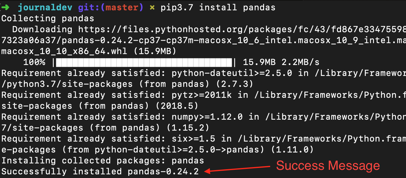
pip3.7 install pandas

To incorporate Pandas and NumPy into your Python script, include the following code snippet:

import pandas as pd
import numpy as np

Since Pandas relies on the NumPy library, it is essential to import this dependency.

Data structures offered in the Pandas module.

Pandas module offers three data structures, which are as stated below:

Series: It is a 1-D size-immutable array like structure having homogeneous data.
DataFrames: It is a 2-D size-mutable tabular structure with heterogeneously typed columns.
Panel: It is a 3-D, size-mutable array.

A DataFrame from the Pandas library.

The DataFrame, which is the most crucial and commonly utilized data structure, serves as a standardized method for data storage. The data in a DataFrame is organized in rows and columns similar to an SQL table or a spreadsheet database. To create a DataFrame object, we have the option to manually input the data or import it from various file types such as CSV, TSV, Excel, or an SQL table. The following constructor can be used for this purpose.

pandas.DataFrame(data, index, columns, dtype, copy)

Here is a brief explanation of the parameters.

data – create a DataFrame object from the input data. It can be list, dict, series, Numpy ndarrays or even, any other DataFrame.
index – has the row labels
columns – used to create column labels
dtype – used to specify the data type of each column, optional parameter
copy – used for copying data, if any

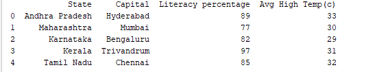
You can create a DataFrame in various ways, such as by using dictionaries or a list of dictionaries. It can also be created from a list of tuples, CSV, Excel file, and so on. To illustrate, let’s execute a basic code to generate a DataFrame from a list of dictionaries.

import pandas as pd
import numpy as np
df = pd.DataFrame({
    "State": ['Andhra Pradesh', 'Maharashtra', 'Karnataka', 'Kerala', 'Tamil Nadu'],
    "Capital": ['Hyderabad', 'Mumbai', 'Bengaluru', 'Trivandrum', 'Chennai'],
    "Literacy %": [89, 77, 82, 97,85],
    "Avg High Temp(c)": [33, 30, 29, 31, 32 ]
})
print(df)

Transferring information from a CSV file to a DataFrame.

We have the option to import a CSV file to create a DataFrame. A CSV file is a text file where each line represents a data record. The values within the record are separated by commas. Pandas offers a convenient function called read_csv() to read the CSV file’s contents and transform them into a DataFrame. For instance, we can have a file named ‘cities.csv’ with information about Indian cities. This CSV file is located in the same directory as our Python scripts. We can import this file by using the following command:

import pandas as pd
data =  pd.read_csv('cities.csv')
print(data)

Our objective is to load and analyze data in order to make informed decisions. Therefore, we can employ any suitable technique for data loading. For this tutorial, we are manually inputting the data into the DataFrame.

Examining data in the DataFrame.

When we run the DataFrame by its name, we can see the complete table. When dealing with real-time datasets that contain thousands of rows, it is necessary to examine data from extensive volumes of datasets for analysis. Pandas offers various helpful functions to inspect specific data. To extract the first n rows, we can use df.head(n), while df.tail(n) allows us to print the last n rows. To illustrate, the code provided below will display the first 2 rows and the last 1 row of the DataFrame.

print(df.head(2))

print(df.tail(1))

1. Obtaining statistical summaries of data.

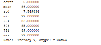
To obtain a statistical summary (which includes count, mean, standard deviation, minimum, maximum, etc.) of the data, we can utilize the df.describe() function. Now, let’s implement this function to present the statistical summary of the “Literacy %” column. To achieve this, we can include the following snippet of code.

print(df['Literacy %'].describe())

2. Arranging data entries in a specific order.

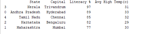
Using the df.sort_values() function, we have the ability to arrange records based on any column. As an illustration, let’s arrange the column “Literacy %” in a descending order.

print(df.sort_values('Literacy %', ascending=False))

3. Cutting through documents

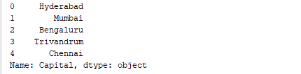
To extract data from a specific column, you can utilize the column name. For instance, when extracting the ‘Capital’ column, we can use:

df['Capital']

or (Only need one alternative)

(df.Capital)

print(df[['State', 'Capital']])

df[0:3]

4. Data filtration

You can also apply column value filters. For instance, the code below filters the columns that have a literacy percentage of over 90%.

print(df[df['Literacy %']>90])

print(df[df['State'].isin(['Karnataka', 'Tamil Nadu'])])

Change the name of the column.

You can utilize the df.rename() function to change the name of a column. This function requires the old column name and the desired new column name as inputs. In this case, we can rename the column ‘Literacy%’ to ‘Literacy percentage’.

df.rename(columns = {'Literacy %':'Literacy percentage'}, inplace=True)
print(df.head())

6. Managing and organizing data efficiently

Native paraphrase:
Data Science includes manipulating data so that it can be utilized effectively by algorithms. Data Wrangling refers to the process of manipulating data, such as combining, categorizing, and joining. The Pandas library offers helpful functions like merge(), groupby(), and concat() to assist in Data Wrangling tasks. To gain a clearer understanding, we will create two DataFrames and demonstrate the functionalities of Data Wrangling.

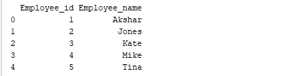
import pandas as pd

d = {  
    'Employee_id': ['1', '2', '3', '4', '5'],
    'Employee_name': ['Akshar', 'Jones', 'Kate', 'Mike', 'Tina']
}
df1 = pd.DataFrame(d, columns=['Employee_id', 'Employee_name'])  
print(df1)

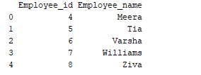
import pandas as pd

data = {  
    'Employee_id': ['4', '5', '6', '7', '8'],
    'Employee_name': ['Meera', 'Tia', 'Varsha', 'Williams', 'Ziva']
}
df2 = pd.DataFrame(data, columns=['Employee_id', 'Employee_name'])  
print(df2)

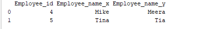
a. Combining

Let’s merge the two DataFrames we made by using the merge() function and matching the values of ‘Employee_id’.

print(pd.merge(df1, df2, on='Employee_id'))

b. Categorizing

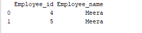
Grouping refers to the act of organizing data into distinct categories. As an illustration, in the given instance, the field labeled “Employee_Name” contains the name “Meera” twice. Therefore, we can group this data by the column titled “Employee_name.”

import pandas as pd
import numpy as np

data = {
    'Employee_id': ['4', '5', '6', '7', '8'],
    'Employee_name': ['Meera', 'Meera', 'Varsha', 'Williams', 'Ziva']
}
df2 = pd.DataFrame(data)

group = df2.groupby('Employee_name')
print(group.get_group('Meera'))

c. Combining together

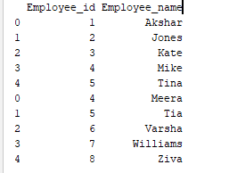
The process of concatenating data involves combining one set of data with another. Pandas offers a function called concat() specifically for merging DataFrames. To illustrate, we can concatenate the DataFrames df1 and df2 using this function.

print(pd.concat([df1, df2]))

One option for paraphrasing the given sentence could be: “Construct a DataFrame by supplying a dictionary consisting of Series.”

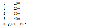
We can make a Series by utilizing the pd.Series() function and supplying it with an array. Now, let’s create a basic Series like this:

series_sample = pd.Series([100, 200, 300, 400])
print(series_sample)

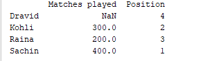
d = {'Matches played' : pd.Series([400, 300, 200], index=['Sachin', 'Kohli', 'Raina']),
'Position' : pd.Series([1, 2, 3, 4], index=['Sachin', 'Kohli', 'Raina', 'Dravid'])}
df = pd.DataFrame(d)
print(df)

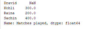
Choosing, including, and removing columns

We have the option to choose a particular column from the DataFrame. To illustrate, if we want to show solely the initial column, we can modify the preceding code as:

d = {'Matches played' : pd.Series([400, 300, 200], index=['Sachin', 'Kohli', 'Raina']),
 'Position' : pd.Series([1, 2, 3, 4], index=['Sachin', 'Kohli', 'Raina', 'Dravid'])}
df = pd.DataFrame(d)
print(df['Matches played'])

d = {'Matches played' : pd.Series([400, 300, 200], index=['Sachin', 'Kohli', 'Raina']),
 'Position' : pd.Series([1, 2, 3, 4], index=['Sachin', 'Kohli', 'Raina', 'Dravid'])}
df = pd.DataFrame(d)
df['Runrate']=pd.Series([80, 70, 60, 50], index=['Sachin', 'Kohli', 'Raina', 'Dravid'])
print(df)

del df['Matches played']

alternatively

df.pop('Matches played')

In summary, to conclude

During this tutorial, we briefly explored the Python Pandas library, conducted practical exercises to demonstrate the capabilities of Pandas in the field of data science, and discussed the various data structures available in the Python library. Source: Official Pandas Website.