画像処理のパート5:算術、ビット演算、およびマスキング
この画像処理シリーズの第5部では、Pythonにおける算術およびビット演算、およびマスキングの詳細について説明します。
こちらのマスク学習の冒険を始める前に、以前の記事を繰り返し読むことをおすすめします。
環境のセットアップを行う
以下のコードは、以下のすべてのアプリケーションで使用されています。巨大なコードブロックを読む必要がないように、ここに含めておきます。
整理を助けます 🙂
# importing numpy to work with pixels
import numpy as np

# importing argument parsers
import argparse

# importing the OpenCV module
import cv2


# initializing an argument parser object
ap = argparse.ArgumentParser()

# adding the argument, providing the user an option
# to input the path of the image
ap.add_argument("-i", "--image", required=True, help="Path to the image")

# parsing the argument
args = vars(ap.parse_args())

# reading the image location through args
# and reading the image using cv2.imread
image = cv2.imread(args["image"])
Pythonを使用した画像の算術演算
算術演算は、画像のさまざまな側面を大幅に向上させることができます。
ライティングやシャドウ、赤、青、緑の色映えの向上に取り組むことができます。
多くのアプリケーションの画像フィルターは、写真を変化させ美化するために同じ方法を使用しています。
では、すべてのコードを始めましょう!
最初に、255以上に制限がかかるか0以下になるかを理解するために、簡単なテストを行うことができます。このテストでは255と0の値が出力されます。
# printing out details of image min, max and the wrap around
print("max of 255 :", str(cv2.add(np.uint8([200]), np.uint8([100]))))
print("min of 0 :", str(cv2.subtract(np.uint8([50]), np.uint8([100]))))

print("wrap around :", str(np.uint8([200]) + np.uint8([100])))
print("wrap around :", str(np.uint8([50]) - np.uint8([100])))
この例では、画像のすべてのピクセルの強度を100増加させています。
# adding pixels of value 255 (white) to the image
M = np.ones(image.shape, dtype="uint8") * 100
added = cv2.add(image, M)
cv2.imshow("Added", added)
cv2.waitKey(0)
これは、NumPyモジュールを使って、私たちの画像と同じサイズの行列を構築し、それに画像を追加することで行われます。
画像を暗くしたい場合、下記のように画像のピクセル値から減算します。
# adding pixels of value 0 (black) to the image
M = np.ones(image.shape, dtype="uint8") * 50
subtracted = cv2.subtract(image, M)
cv2.imshow("Subtracted", subtracted)
cv2.waitKey(0)
これにより、元の画像の明るさや暗さを変えたバリエーションが2つ提供されます。
ビット演算
画像のマスキングを試みる際には、ビット演算をよく使用します。
OpenCVのこの機能により、私たちに関連する画像の一部をフィルタリングすることができます。
セットアップの準備
ビット演算をするためには、まず操作を行うための2つの変数または画像が必要です。
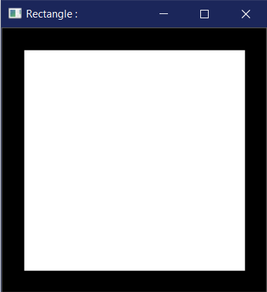
では、ビットごとの演算ができるように、ビットごとの正方形とビットごとの円を作りましょう。
ビット演算を行うためには、画像は白と黒である必要があります。
# creating a square of zeros using a variable
rectangle = np.zeros((300, 300), dtype="uint8")
cv2.rectangle(rectangle, (25, 25), (275, 275), 255, -1)
cv2.imshow("Rectangle : ", rectangle)

# creating a circle of zeros using a variable
circle = np.zeros((300, 300), dtype="uint8")
cv2.circle(circle, (150, 150), 150, 255, -1)
cv2.imshow("Circle : ", circle)
受け取る出力画像は、こちらのように見えるべきです。 (Uketoru shutsuryoku gazō wa, kochira no yō ni mieru beki desu.)
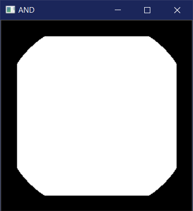
「AND」演算子を使って結合してください。
ビット演算加算は、2つの異なる画像の加算を参照し、画像の各ピクセルにAND演算を適用して表示することを指します。
# the bitwise_and function executes the AND operation
# on both the images
bitwiseAnd = cv2.bitwise_and(rectangle, circle)
cv2.imshow("AND", bitwiseAnd)
cv2.waitKey(0)
円と四角形のビットワイズ加算によって、以下のような出力が得られます。
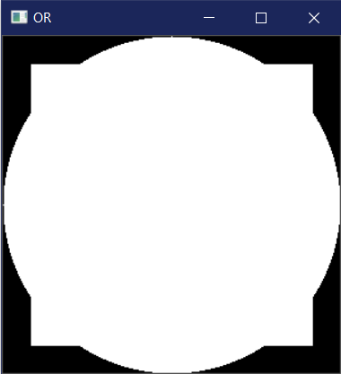
OR 操作を使用した場合の選択肢が与えられた場合
ビット単位の論理和は、各画素に対してOR演算を行った結果として、二つの画像の積を提供します。
# the bitwise_or function executes the OR operation
# on both the images
bitwiseOr = cv2.bitwise_or(rectangle, circle)
cv2.imshow("OR", bitwiseOr)
cv2.waitKey(0)
操作のビット毎の論理和を実行する際に、以下のような結果が得られるはずです。
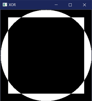
XOR 演算による排他性
cv2モジュールが提供する別の操作は、bitwise_xor関数を通じて使用できるXOR操作です。
# the bitwise_xor function executes the XOR operation
# on both the images
bitwiseXor = cv2.bitwise_xor(rectangle, circle)
cv2.imshow("XOR", bitwiseXor)
cv2.waitKey(0)
NOT演算子を使った否定
最後に、ビットごとの否定操作を行うためのbitwise_not関数があります。
NOT演算子は、何も追加や減算する必要なく、単一の画像のみが必要です。
しかし、ここでもそれをまだ使用しているのは、それも選択肢の一つです。
# the bitwise_not function executes the NOT operation
# on both the images
bitwiseNot = cv2.bitwise_not(rectangle, circle)
cv2.imshow("NOT", bitwiseNot)
cv2.waitKey(0)
この場合、円は四角形の内側にあり、そのため見えません。
PythonのOpenCVを使用した画像のマスキング。
マスキングは画像処理において使用され、関心のある部分、つまり私たちが興味を持っている画像の一部を出力するために使われます。
イメージの必要のない部分を取り除くために、ビット演算をマスキングによく利用します。
さあ、マスキングを始めましょう!
画像のマスキングプロセス
マスキングには3つのステップがあります。
-
- 原画像と同じサイズの黒いキャンバスを作成し、マスクと名付けます。
-
- 画像内に任意の図形を描画し、白い色を与えることでマスクの値を変更します。
- 画像とマスクの間でビット単位の加算操作を行います。
同じプロセスに従って、いくつかのマスクを作成し、それらを画像に使用しましょう。
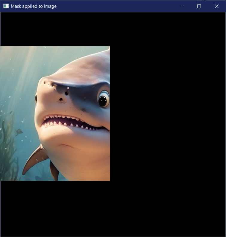
最初に、長方形のマスクで作業しましょう。
# creating a mask of that has the same dimensions of the image
# where each pixel is valued at 0
mask = np.zeros(image.shape[:2], dtype="uint8")

# creating a rectangle on the mask
# where the pixels are valued at 255
cv2.rectangle(mask, (0, 90), (290, 450), 255, -1)
cv2.imshow("Mask", mask)

# performing a bitwise_and with the image and the mask
masked = cv2.bitwise_and(image, image, mask=mask)
cv2.imshow("Mask applied to Image", masked)
cv2.waitKey(0)
では、さっそく円形のマスクで試してみましょう。
# creating a mask of that has the same dimensions of the image
# where each pixel is valued at 0
mask = np.zeros(image.shape[:2], dtype="uint8")

# creating a rectangle on the mask
# where the pixels are valued at 255
cv2.circle(mask, (145, 200), 100, 255, -1)
cv2.imshow("Mask", mask)

# performing a bitwise_and with the image and the mask
masked = cv2.bitwise_and(image, image, mask=mask)
cv2.imshow("Mask applied to Image", masked)
cv2.waitKey(0)
すべてがうまくいけば、私たちはこんな風に見えるような出力を受け取るはずです。
結論
ついに画像処理の中核に入ります。ビット演算とマスキングの理解は重要です。
私たちには、興味のある部分だけを取り込んだり、画像の一部をブロックしたりするために役立ちます。だから、かなり便利な概念です。
私たちは適度なスピードで進んでいますが、もし終わりに早送りしたい場合は、どうぞご自由に!
以下は、OpenCVと顔認識について詳しく知ることができる記事と、AndroidとCameraX OpenCVのJava実装を紹介しています。
参考文献
- Official OpenCV Website
- Introduction to starting out with OpenCV
- My GitHub Repository for Image Processing
- Arithmetic Operations Code
- Bitwise Operations Code
- Masking Code